Astronomy Research
Learn about the various research that has taken place at Luther.
Along with stopping power, position resolution and sensitivity, energy resolution is one of the key features of any x-ray detector. Energy resolution refers to a detector’s ability to determine precisely the energy of any incident x-ray. Improved energy resolution yields cleaner spectra of objects such as neutron stars. These cleaner spectra can then be used to build improved models of the interactions occurring in the magnetospheres of these highly magnetic stellar remnants.
Much of the work that I did as a graduate student and postdoc was aimed at improving the energy resolution of a xenon gas scintillation proportional counter designed for use in x-ray astronomy in the 20 to 300 keV energy band. Using plane parallel proportional counters with CsI photocathodes and low pressure methane gas, we were able to achieve an ultimate energy resolution within a factor of two of the expected theoretical limit. The primary limiting factor in energy resolution should come from Fano fluctuations in the electron drift cloud resulting from the photoelectric absorption of the incident x-ray. You can find our results published in SPIE Conference Proceedings, 2806, pp. 361-371, 1996. A good deal of the work I have done with students has been in attempting to track down the cause of the two worsening factors of the energy resolution.
Lately, this work has led us to search for infrared emission from xenon gas. Traditionally, vacuum ultraviolet scintillation emission has been used to form the basis of xenon scintillation detectors. We decided that if infrared emission existed it might be a new channel we could use to get information on the incident x-ray’s energy. We set about trying to determine if xenon did scintillate in the infrared and if that infrared emission could be used to form the basis of an x-ray or particle detector. We searched for emission around the known atomic xenon emission lines at 823 nm and 828nm. We found that infrared scintillation did, indeed, exist and its yield increased as the xenon pressure was decreased below one atmosphere. The xenon yield did not prove to be large enough to meet our needs for an astronomical x-ray detector but the yield was sufficient to perhaps be of interest to people working in other areas. The results can be found in the journal Nuclear Instruments and Methods.
We have been measuring the “apparent brightness” of more than 1600 stars in a single field since 2003, with occasional stops to observe other fields. We acquire hundreds or thousands of images of a rich star field in a given night. This work should prove useful for the study of everything from meteors to near-earth asteroids to variable stars and foreground objects passing between us and a distant star. Much of our current effort focuses on the approximately 60 new semi-regular variable stars we have discovered in this field. We are looking for evidence of multiple pulsation modes and secular evolution in these stars. We also monitor half a dozen eclipsing binary stars in the field, looking for subtle changes in the orbital periods of these systems and we search for rare stellar flares.
Students are an active part of this ongoing research work, leading to dozens of individual student research projects.
Our Data
Since 2003 we have acquired more than half a million images of a field half a degree square, containing the open star cluster M23. We shoot unfiltered images that are a few seconds in duration. These unfiltered images provide the greatest signal-to-noise ratio in the shortest time while offering unique challenges in frame normalization and calibration. We occasionally acquire images from other fields but our primary focus has been the M23 field to which we return season after season. This effort has led to a data set uniquely able to provide information on the stability of stellar signals on timescales ranging from seconds to decades.
View a table summarizing recent observations
Long-period Variable Stars
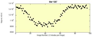
By the end of the 2014 data season we had indisputable evidence of variability in about 60 of the approximately 1600 stars in our field of view. The vast majority of these stars are long-period variable stars and the majority of these variables would be classed as semi-regular variables. Most of these stars vary on timescales of a few tens of days to a few hundred days and have amplitudes of variation between about 0.2 and 0.5 magnitude. We are slowly deciphering the properties of these stars. Most are multi-periodic with two or more oscillation modes excited. We are searching for hints of even longer oscillation modes and for evidence of whether these stars are on average getting brighter or dimmer. We are also interested in the stability of the different oscillation modes in a given star as well as potential outbursts these stars might show. In addition to these variables we are monitoring dozens more stars that are likely, but not yet indisputably, long-period variables. Here we have two images of a star we know affectionately as Star 356, taken several months apart. Yup, it got brighter.
Eclipsing Binary Systems
We have found 6 stars in our field to be eclipsing binary systems, where one star periodically passes in front of the other from our vantage point. When this “eclipsing” occurs the apparent single star that we see gets dimmer. Timing these eclipses allows us to test several properties of the system including the rate of mass loss from the system, mass transfer from one star to the other, how the magnetic fields of the stars interact with one another and whether an unseen third star inhabits the system. Most of the eclipsing binaries we see are very close to one another, almost touching, with orbital periods on the order of a day or less. Shown below is a signal versus time graph (a light curve) for an eclipse in one of these systems.
Flare Events and Other Rare Transients
When we started this work so many years ago we were most keenly interested in the very shortest time scale changes that might occur. Such a blip might arise from an outer solar system object blocking the light of a star briefly as it passes or a black hole microlensing a background star, causing it to appear brighter. This is long haul work with plenty of statistical testing and re-testing. We keep at it, searching for a few needles in very large haystacks. Of course, we are also sensitive to classical stellar flare events and a few apparent flares have appeared.
Data Analysis Graphs
In our work of better understanding the stars in our field and how they are changing, dramatically of subtly, we generate many graphs. During my (Professor Jeff Wilkerson’s) most recent sabbatical year I generated an average of four graphs per day for example. These were just the graphs I made by hand, not ones automatically machine-generated. We collect some of these graphs here to tell a little bit of the story of our work. These graphs are sorted into categories that may change from time-to-time.
Pulsating Variables
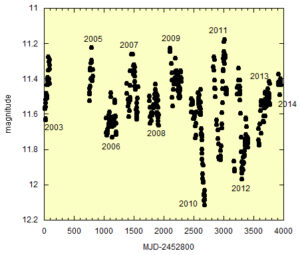
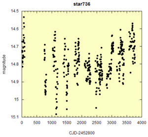
A video that shows the light curve of the star described below evolving year to year. Most of our pulsating variable stars are red with periods between about 80 days and 400 days. Many have very long secondary periods of maybe thousands of days. One star is not as red as the others and has a significantly shorter period of variation, as might be more typical of, say, a Cepheid. Our best-fit period for this star is 14.898 days. Shown below is a light curve from late summer 2010.
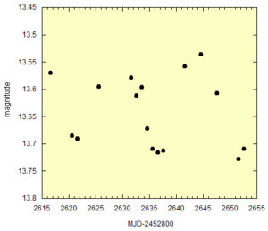
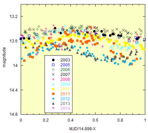
The above light curve comes from a data-friendly stretch when we got 16 nights of data in 36 days. This light curve is evolving more strongly than most. Below is a phase diagram folded on the 14.898 day period. From 2003 to 2014 the amplitude of variation grew while the star got fainter on average. There is some evidence that the amplitude is getting smaller again – a very interesting star.
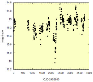
Above we see a light curve of a semi-regular variable star that shows a sudden increase of variability amplitude in 2010, when the amplitude more than doubled. 2013 into 2014 it appears that the star has settled back into low-amplitude mode. It should be noted that the 2014 data appear prior to passing photometric quality tests and some nights might be removed later. The pre-outburst and post-outburst sections of the light curve are shown in more detail below.

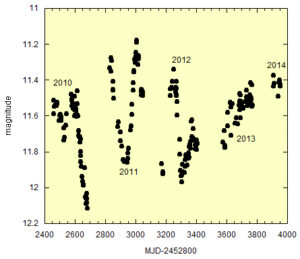
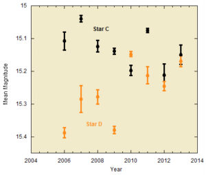
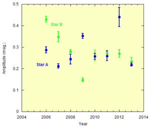
In the section below we looked at changes in mean magnitude (“brightness”) and amplitude for two semi-regular variable stars in our field. Above is an annual mean magnitude graph for two more stars. Star C is consistent with having gotten fainter and Star D looks to have brightened. We started down this path wondering if these SR stars are on average getting brighter or fainter as a group. With the four we have looked at oh so briefly here there is no suggestion of one or the other. We are also surprised by the size of the changes we have seen in these stars. Below is the graph of amplitude as a function of year for these stars. As with the stars in the next section the amplitudes are messier and harder to make any claims about. Another 20 to 40 stars have reasonable periods to do this work with. We shall see what arises.
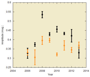
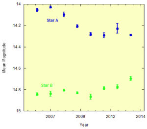
The mean magnitude of two semi-regular variables over each of the past 8 observing seasons. We look for evidence of long-term evolution in these systems. These two stars (of the ~60 SR stars in our study) show particularly large changes in these 8 years. Are the changes due to very long period oscillations? Are they related to equipment changes we made? The change in Star A is consistent with a single step down and the change in Star B is consistent with a more recent step up. It is also possible that Star A is showing a steady decrease in light with oscillations around that decrease. To create these light curves we averaged (carefully due to uneven phase sampling) over shorter term variations of timescales 150 to 250 days or so. We are working on the questions raised here and more but it simply might require following these systems for another decade. The amplitudes of variation of these stars by year are shown in the figure below. Any change in amplitude is less clear although a case could be made for a meaningful decrease in the amplitude of Star B.
A multi-periodic semi-regular variable that shows an apparent decrease in amplitude and a change in mean magnitude over the past decade. One question we are trying to answer is if such changes have been common and of similar sign for the 60 or so semi-regulars in our field and whether these changes are monotonic or cyclic.
A pulse in a variable star
Some of our variable stars show sudden “pulses” in signal variation and then settle back into relatively low amplitude variations. How common are these pulses? What are these pulses? Below is a “close up” of the time around the pulse.
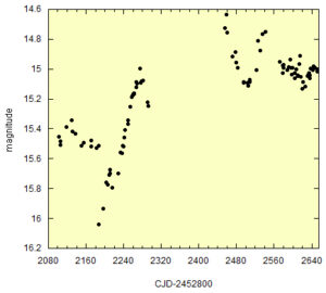
A close look at a pulse in a variable star.
Eclipsing Binary Star Systems
We have found about half a dozen eclipsing binary star systems in our field of view. These are systems containing two stars with separations sufficiently small so that they appear as a single star to us. The orbits of these stars are oriented so that periodically one star passes in front of the other star (from our vantage point). When one star passes behind the other star its light is lost and the system appears to get dimmer. We see the star get dimmer until maximum occultation, remain at minimum light while at maximum occultation and then the light from the system grows again until both stars are once again seen fully.
A different system has an eclipse duration so long that we never see a a complete eclipse process in a night. This system has a period of almost exactly 5.50 days so that we see eclipses every 11 nights. We were fortunate to have clear nights on March 25 and April 5, 2015.
A third system has a very short period (about six hours) and we only see a partial eclipse so that when the system reaches minimum light it immediately begins getting brighter.
Flare-like Events
An apparent brightening of a star in our field over about a 90 minute time span. We make millions of measurements of individual star brightness and apparent fluctuations on multiple timescales are common. For nearly all these a non-astronomical origin for the increase in measured signal can be found – bleed in from a neighboring star image, a passing satellite, odd interactions with the edge of the field of view. Occasionally, the source of the increased signal will be astronomical but not of particular interest to us for this project, such as when the image of an asteroid is aligned with the background star image. For a few, such as in the case above, no obvious source of the excess signal has been found and the possibility of a more interesting source for the event remains open for the time being.
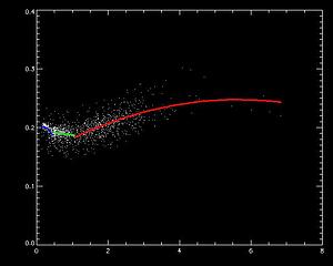
Due to time-varying atmospheric scatter and absorption we need to normalize our images. One of the biggest challenges in this work comes from the images being unfiltered so that we achieve the maximum signal-to-noise ratio in the shortest time, aiding our efforts to find very short flare events. We had achieved normalizations that were sufficient for most of our efforts by simply forcing the median stellar signal to remain constant frame-to-frame. This method is blind to stellar color but the atmospheric scattering certainly is not as evidenced by the blue sky. The histograms in the sections below this one were made with this older frame normalization method. One reason we have been using this normalization method is efficiency. We have, after all, made about one billion individual star brightness measurements over the past several years. As we began to explore ever more subtle effects, such as secular variation in pulsating stars, it became imperative to improve our photometry by incorporating stellar color in the normalization. In summer 2015 we worked to fit curves to plots of measured star signal divided by measured star signal in a reference image as a function of the measured color index of the stars. A sample graph is shown here.
Once we applied this new frame normalization to our 10+ years of data we saw the following transformation in the light curve of one star, new normalization on the right/below:
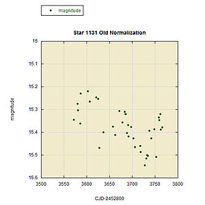
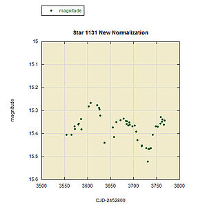
The improvement was pretty stark. This work allowed us to move about 20 stars from “likely variable” to “variable.” All of these stars were relatively low amplitude, short period pulsating stars, allowing us a much richer data set for the variable star population studies we are doing in our field.
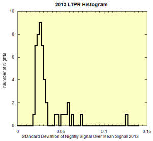
A measure night-to-night signal scatter in 2013.
A histogram of night-to-night signal scatter in 2013 for the 800 brightest stars in the field with the known variable stars removed. The statistic used in the histogram is the standard deviation of the distribution of each star’s nightly measured mean signal divided by the mean signal for the entire observing season. For most of our work we reject the outlying nights with relatively large values of this ratio.
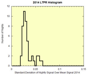
Above is the same histogram for the 2014 data. The distribution is similar to that seen in 2013, as we might expect. Note that the plot was scaled to match the prior year and one night was cut out, falling just to the right of the data shown above. Choosing where to make the cut to eliminate poor photometry nights in any year is essentially arbitrary. We have clear evidence that the poorest photometry nights lead to outlying points on our variable star light curves but exactly how bad and when an “outlier” becomes an “outlier” is (at least somewhat) open for interpretation. What is certain is that when we make a cut we need to keep every night below the cut and remove every night above the cut, no exceptions. Looking back I see that we chose 0.050 (5 percent) as the cut in 2013. With nothing to suggest strongly otherwise we used that same cut in 2014, eliminating 7 of the 47 data nights. We could have made an argument for using 0.035 and keeping only the “main peak” but we decided that we preferred to have those extra five nights in the data set. However, we remain aware that we need to be wary of making any big claims that rely heavily on those nights.
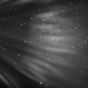
Scattered Moon
This image, taken prior to focusing for the evening, shows what happens when an 80 percent full moon lies 10 degrees from the cluster we are studying. You gotta know when to fold ’em.
Shutter Failure
When a shutter fails it typically does so by failing to close completely between images. The result is that the center of the frame is overexposed. Above is a dark image taken after a suspected shutter failure. Dark images are used to subtract out pixel noise. One collects charge in each pixel for some time (often a time equal to an exposure duration) while the shutter is closed. That is, the shutter is never told to open for a dark frame. The resulting signal can then be subtracted from the raw images since the counts are due to noise the camera is generating. I don’t think the camera shutter was closed all the way when the above dark frame was shot, do you?
2022
- “Developing software and building an analysis program to allow research project continuity with a new replacement digital camera” with Suman Chapai and Minh Nguyen, Luther College, 2022.
- “Initial assessment of linear tracks in 18 years of images of a half-degree square field centered on open star M23 near the direction of the Galactic center and lying near the ecliptic” with Isaac Roberts, Luther College, 2022.
2021
- “Investigating the role of atmospheric scintillation, stellar characteristics and image alignment on photometric resolution limits achievable from a deep-atmosphere site” with Owen Johnson, Luther College, 2021.
- “Assessing how the definition of ‘range of variance’ impacts the results of studies of evolution in long-period pulsating variable stars” with Isaac Roberts, Luther College, 2021.
- “Searching for evidence of recent period and amplitude variations in short-period partially-eclipsing binary star system” with Darren Kremer Luther College, 2021.
- “Determining the physical and statistical significance of apparent outburst events in mono-periodic long-period pulsating variable stars” with Thandeka Chaka, Luther College, 2021.
2020
- “Determining the spatial location of long-period pulsating variable stars in the field of open star cluster M23” with Owen Johnson, Luther College, 2020.
- “Assessing the relative importance of stellar color and stellar neighbors to systemic errors in stellar photometry of a crowded field” with Suman Chapai, Mae Cody, Darren Kremer, Jacob Larson, Minh Nguyen and Sam Wilson, Luther College, 2020.
2019
- “Assessment of the feasibility of using the R-I color index of stars for intra-night frame normalization to improve short-term photometric resolution” with Mae Cody, Luther College, 2019.
- “Developing efficient data storage structures for a long-term data-intensive stellar photometric monitoring research project” with Blake Krapfl, Luther College, 2019.
- “Dramatic Amplitude Evolution of a Potential Cepheid Variable Star” with Rahul Bagga, Luther College, 2019.
- “Period Evolution of Partially Eclipsing Binary System” with Owen Johnson, Luther College, 2019.
2018
- “Searching for evidence of a third body in a partially eclipsing binary system” with Torger Jystad, Luther College, 2018.
- “Assessing the feasibility of using annular aperture photometric approach to background subtraction in a crowded stellar field” with Alex Pigarelli, Luther College, 2018.